Black-Scholes Option Model
The Black-Scholes Model was developed by three academics: Fischer Black, Myron Scholes and Robert Merton. It was 28-year old Black who first had the idea in 1969 and in 1973 Fischer and Scholes published the first draft of the now famous paper The Pricing of Options and Corporate Liabilities.
The concepts outlined in the paper were groundbreaking and it came as no surprise in 1997 that Merton and Scholes were awarded the Noble Prize in Economics. Fischer Black passed away in 1995, before he could share the accolade.
The Black-Scholes Model is arguably the most important and widely used concept in finance today. It has formed the basis for several subsequent option valuation models, not least the binomial model.
What Does the Black-Scholes Model do?
The Black-Scholes Model is a formula for calculating the fair value of an option contract, where an option is a derivative whose value is based on some underlying asset.
In its early form the model was put forward as a way to calculate the theoretical value of a European call option on a stock not paying discrete proportional dividends. However it has since been shown that dividends can also be incorporated into the model.
In addition to calculating the theoretical or fair value for both call and put options, the Black-Scholes model also calculates option Greeks. Option Greeks are values such as delta, gamma, theta and vega, which tell option traders how the theoretical price of the option may change given certain changes in the model inputs. Greeks are an invaluable tool in portfolio hedging.
Black-Scholes Equation
Call Option = 
Where:
Given Put Call Parity:
The price of a put option must therefore be:
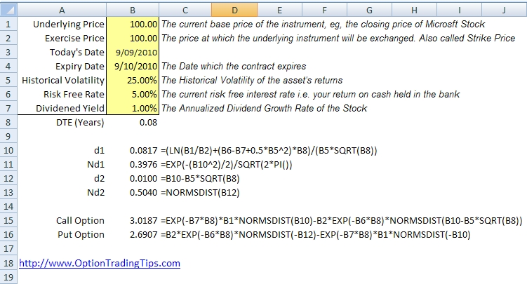
Black-Scholes Excel
Black-Scholes VBA
Function dOne(UnderlyingPrice, ExercisePrice, Time, Interest, Volatility, Dividend)
dOne = (Log(UnderlyingPrice / ExercisePrice) + (Interest - Dividend + 0.5 * Volatility ^ 2) * Time) / (Volatility * (Sqr(Time)))
End Function
Function NdOne(UnderlyingPrice, ExercisePrice, Time, Interest, Volatility, Dividend)
NdOne = Exp(-(dOne(UnderlyingPrice, ExercisePrice, Time, Interest, Volatility, Dividend) ^ 2) / 2) / (Sqr(2 * 3.14159265358979))
End Function
Function dTwo(UnderlyingPrice, ExercisePrice, Time, Interest, Volatility, Dividend)
dTwo = dOne(UnderlyingPrice, ExercisePrice, Time, Interest, Volatility, Dividend) - Volatility * Sqr(Time)
End Function
Function NdTwo(UnderlyingPrice, ExercisePrice, Time, Interest, Volatility, Dividend)
NdTwo = Application.NormSDist(dTwo(UnderlyingPrice, ExercisePrice, Time, Interest, Volatility, Dividend))
End Function
Function CallOption(UnderlyingPrice, ExercisePrice, Time, Interest, Volatility, Dividend)
CallOption = Exp(-Dividend * Time) * UnderlyingPrice * Application.NormSDist(dOne(UnderlyingPrice, ExercisePrice, Time, Interest, Volatility, Dividend)) - ExercisePrice * Exp(-Interest * Time) * Application.NormSDist(dOne(UnderlyingPrice, ExercisePrice, Time, Interest, Volatility, Dividend) - Volatility * Sqr(Time))
End Function
Function PutOption(UnderlyingPrice, ExercisePrice, Time, Interest, Volatility, Dividend)
PutOption = ExercisePrice * Exp(-Interest * Time) * Application.NormSDist(-dTwo(UnderlyingPrice, ExercisePrice, Time, Interest, Volatility, Dividend)) - Exp(-Dividend * Time) * UnderlyingPrice * Application.NormSDist(-dOne(UnderlyingPrice, ExercisePrice, Time, Interest, Volatility, Dividend))
End Function
You can create your own functions using Visual Basic in Excel and recall those functions as formulas within your chosen workbook. If you want to see the code in action complete with Option Greeks, download my Option Trading Workbook.
The above code was taken from Simon Benninga's book Financial Modeling, 3rd Edition. I highly recommend reading this and Espen Gaarder Haug's The Complete Guide to Option Pricing Formulas
. If you're short on option pricing formulas texts, these two are a must.
Model Inputs
From the formula and code above you will notice that six inputs are required for the Black-Scholes model:
- Underlying Price (price of the stock)
- Exercise Price (strike price)
- Time to Expiration (in years)
- Risk Free Interest Rate (rate of return)
- Dividend Yield
- Volatility
Out of these inputs, the first five are known and can be found easily. Volatility is the only input that is not known and must be estimated.
Black-Scholes Volatility
Volatility is the most important factor in pricing options. It refers to how predictable or unpredictable a stock is. The more an asset price swings around from day to day, the more volatile the asset is said to be. From a statistical point of view volatility is based on an underlying stock having a standard normal cumulative distribution.
To estimate volatility, traders either:
- Calculate historical volatility by downloading the price series for the underlying asset and finding the standard deviation for the time series. See my Historical Volatility Calculator.
- Use a forecasting method such as GARCH.
Implied Volatility
By using the Black-Scholes equation in reverse, traders can calculate what's known as implied volatility. That is, by entering in the market price of the option and all other known parameters, the implied volatility tells a trader what level of volatility to expect from the asset given the current share price and current option price.
Assumptions of the Black-Scholes Model
1) No Dividends
The original Black-Scholes model did not take into account dividends. Since most companies do pay discrete dividends to shareholders this exclusion is unhelpful. Dividends can be easily incorporated into the existing Black-Scholes model by adjusting the underlying price input. You can do this in two ways:
- Deduct the current value of all expected discrete dividends from the current stock price before entering into the model or
- Deduct the estimated dividend yield from the risk-free interest rate during the calculations.
You will notice that my method of accounting for dividends uses the latter method.
2) European Options
A European option means the option cannot be exercised before the expiration date of the option contract. American style options allow for the option to be exercised at any time before the expiration date. This flexibility makes American options more valuable as they allow traders to exercise a call option on a stock in order to be eligible for a dividend payment. American options are generally priced using another pricing model called the Binomial Option Model.
3) Efficient Markets
The Black-Scholes model assumes there is no directional bias present in the price of the security and that any information available to the market is already priced into the security.
4) Frictionless Markets
Friction refers to the presence of transaction costs such as brokerage and clearing fees. The Black-Scholes model was originally developed without consideration for brokerage and other transaction costs.
5) Constant Interest Rates
The Black-Scholes model assumes that interest rates are constant and known for the duration of the options life. In reality interest rates are subject to change at anytime.
6) Asset Returns are Lognormally Distributed
Incorporating volatility into option pricing relies on the distribution of the asset’s returns. Typically, the probability of an asset being higher or lower from one day to the next is unknown and therefore has a 50/50 probability. Distributions that follow an even price path are said to be normally distributed and will have a bell-curve shape symmetrical around the current price.
It is generally accepted, however, that stocks – and many other assets in fact – have an upward drift. This is partly due to the expectation that most equities will increase in value over the long term and also because a stock price has a price floor of zero. The upward bias in the returns of asset prices results in a distribution that is lognormal. A lognormally distributed curve is non-symmetrical and has a positive skew to the upside.
Geometric Brownian Motion
The price path of a security is said to follow a geometric Brownian motion (GBM). GBMs are most commonly used in finance for modelling price series data. According to Wikipedia a geometric Brownian motion is a “continuous-time stochastic process in which the logarithm of the randomly varying quantity follows a Brownian motion". For a full explanation and examples of GBM, check out Vose Software.
61 Comments
Peter January 5th, 2015 at 5:13am
Hi Bruce,
No, that shouldn't be the case. I was just about to reply with that, but then checked a few scenarios using my spreadsheet to see how close it was...with the volatility at 30% an ATM option comes close to this...but OTM/ITM options are way out. Same when the vol is higher or lower than 30%. Not sure why this happens.
Did you read this somewhere or did someone else mention this to be the case?
Bruce January 4th, 2015 at 3:46pm
Should the option price equal the IV times the vega?
Peter March 4th, 2014 at 4:45am
Hi Satya,
Ah no, I only have the binomial model and the BS. If you find some good examples of the others please let me know so I can put them here too!
Satya March 4th, 2014 at 3:15am
Peter,
Do you have models for the BS model only or you have them for other models like the Heston-Nandi or the Hull-White Models? If you do, could you share them? i need them for a my project.
Peter April 26th, 2012 at 5:46pm
Ah ok, no worries, glad it worked out.
Mario Marinato April 26th, 2012 at 7:05am
Hi, Peter. When I entered the various possible values they all gave me the same fair price.
Asking for help on another site*, I got a hint that led me to the discovery of my mistake: my B&S formula was rounding the fair prices below 0.01 to 0.01.
Thus, with out-of-the-money options, their fair prizes where always below 0.01 given a wide range of volatilities, and my formula was returning 0.01 to all of them.
I changed the formula and everything came into place.
Thanks for your attention.
Best regards from Brazil.
* Precision & Implied Volatility
Peter April 25th, 2012 at 10:29pm
Hi Mario,
Sounds like you're not allowing enough time to get to the right implied volatility.
What happens when you re-enter those other volatility values back into B&S...you will get a different theoretical price, right?
Mario Marinato April 24th, 2012 at 9:37am
Hi,
I'm developing a software to calculate the implied volatility of an option using the Black & Scholes formula and a trial-and-error method. The implied volatility values I get are correct, but I noticed that they are not the only possible ones.
For example, with a given set of parameters, my trial-and-errors lead me to an implied volatility of 43,21%, which, when used on B&S formula, outputs the price I started with. Great!
But I realized this 43,21% value is just a fraction of a much wider range of possible values (let's say, 32,19% - 54,32%).
Which value should I, then, pick as the 'best' one to show to my user?
Best regards,
Peter December 18th, 2011 at 3:56pm
Hi Utpaal, yes, you can use whatever price you like to calculate the implied volatility - just enter the closing prices in the "market price" field.
Peter December 18th, 2011 at 3:53pm
Hi JK, you can find spreadsheets for pricing American options on the binomial model page.
Add a Comment